How can a repeating exoplanet transit be detected in a noisy light-curve dataset without mistaking it for proof of a planet?
01 // Question
Which trial period best aligns repeated shallow dips in a noisy synthetic light curve, and what evidence would still be needed before calling the signal a planet?
Every numeric value in the activity dataset is invented for instruction and is not NASA telescope data or a discovered planet. Recovering an injected repeating dip demonstrates a method, not a real exoplanet detection.
02 // Variables
Independent
Trial period used to group the same time-ordered observations by phase- 7-hour trial period
- 8-hour trial period
- 9-hour trial period
- same 24 synthetic flux points for every test
Dependent
How well a repeated shallow dip aligns in phase relative to the out-of-transit baseline- mean normalized flux in transit-phase bins
- estimated dip depth relative to baseline
- number of repeated dips that align and note of scatter or gaps
03 // Hypothesis
IF the same noisy measurements are folded at the period used to create their repeated synthetic dips, THEN the dips will line up at one phase and form a clearer average decrease than when folded at nearby incorrect periods, BECAUSE phase folding places observations from repeated cycles at the same relative orbital phase, allowing a recurring pattern to reinforce while uncorrelated noise is less aligned.
04 // Procedure
1. Start with an explicitly synthetic dataset
Use the 24 time-and-flux values in the data table as if they were one short telescope sequence. The values are synthetic: a shallow dip was inserted near the same phase about every eight hours, then small scatter was added. Do not describe this table as a NASA observation or a real planet. Keep the raw values visible throughout the analysis.
2. Plot time against normalized brightness
Make a scatter plot with time in hours on the horizontal axis and normalized flux on the vertical axis. Transit-like events appear as small decreases, not brightening. Mark uncertainty or outlying points; do not connect large gaps with a line that implies continuous observation. Note that the small visual changes are deliberately hard to see at first.
3. Fold the same curve at three trial periods
For each trial period, calculate phase = (time modulo period) ÷ period. Use the same phase bins for all three tests and calculate the mean flux in each bin. Compare whether the lowest points cluster at one phase across multiple cycles. An eight-hour period is the injected pattern, but students should justify it by alignment, not by being told the answer before plotting.
4. Estimate depth and compare scatter
Choose the in-transit phase window before scoring periods. Estimate transit depth as the out-of-transit baseline mean minus the mean inside that window, expressed as a fraction of baseline. Also report the number of points and their spread; a deeper apparent dip based on one point or one cycle is weaker evidence than a repeated, aligned pattern. Do not silently remove data to improve the score.
5. Test how noise removal can change the signal
For a real Kepler or TESS light curve, slow instrumental trends, scattered light, stellar rotation, flares and gaps may require correction. Compare the raw and corrected series and preserve a copy of each. A detrending window that is too short can flatten or erase a long or shallow transit; a window that is too long can leave background trends. NASA's TESS tutorial compares correction methods because no one correction is right for every star and timescale.
6. Call it a candidate and list the next checks
A repeating dip is a transit-like candidate, not proof of a planet. Eclipsing binary stars, blended background sources, stellar variability, instrumental events and data-processing artifacts can mimic or distort a signal. Professional vetting examines the pixel data, odd/even events, secondary eclipses, centroid shifts, statistical significance and follow-up observations. Report the method, assumptions and uncertainty before making a claim.
Materials // Prepare the bench
- the 24-row synthetic flux table from this article
- spreadsheet or graph paper
- calculator
- phase-folding worksheet with candidate periods 7, 8 and 9 hours
05 // Data table
| Time (h) | Synthetic normalized flux | Time (h) | Synthetic normalized flux |
|---|---|---|---|
| 0 | 1.000 | 12 | 0.993 |
| 1 | 0.999 | 13 | 0.997 |
| 2 | 1.001 | 14 | 1.001 |
| 3 | 0.996 | 15 | 0.999 |
| 4 | 0.994 | 16 | 0.999 |
| 5 | 0.999 | 17 | 1.001 |
| 6 | 1.000 | 18 | 1.000 |
| 7 | 1.001 | 19 | 0.994 |
| 8 | 1.001 | 20 | 0.995 |
| 9 | 1.000 | 21 | 0.998 |
| 10 | 0.999 | 22 | 0.999 |
| 11 | 0.995 | 23 | 1.001 |
Compare candidate periods using the same scoring rules
| Trial period | Expected phase result | What to report | Caution |
|---|---|---|---|
| 7 hours | Repeated dips drift across phase bins | Depth, scatter, number of cycles aligned | A single dip may look convincing by chance |
| 8 hours | Injected dip phases align across three cycles | Depth, scatter, number of cycles aligned | This recovers a known synthetic input, not a discovered planet |
| 9 hours | Repeated dips drift across phase bins | Depth, scatter, number of cycles aligned | A wrong period can partially align only a subset |
A transit-like dip has several possible causes
| Possible cause | Why it can look transit-like | Useful follow-up |
|---|---|---|
| Planet transit | A planet blocks some starlight at repeated orbital phases | Check repetition, depth shape, stellar properties and independent evidence |
| Eclipsing binary or blended star | A star can eclipse another star or contaminate the target aperture | Inspect odd/even depths, secondary events, pixels, centroid and spectra |
| Stellar variability | Spots, rotation or flares change brightness over time | Compare timescales, color, repeated patterns and multiple observations |
| Instrument or processing artifact | Scattered light, motion, gaps or detrending can create or erase a dip | Review raw/corrected light curves, quality flags and pixel-level data |
06 // What to expect
The 8-hour folding best aligns the synthetic dips near the same phase; the 7- and 9-hour trials spread them more broadly.
The estimated depth is small compared with baseline flux, so plotting, repeated events, noise and selected phase windows matter to interpretation.
The data demonstrate recovery of a deliberately inserted signal only. A real transit-like signal needs pipeline vetting and follow-up before it can be described as a confirmed planet.
07 // Lab notes
- All 24 table values are synthetic teaching data with an injected approximately 8-hour pattern. They are not measured values from Kepler, TESS, NASA, or any known star.
- Do not equate one dip or a strong periodogram peak with planet confirmation. Kepler validation products evaluate transit-like events with multiple diagnostic tests and false-positive checks.
- Detrending is a scientific choice: corrections can remove instrumental patterns but can also attenuate a real transit if the correction timescale overlaps the signal.
08 // Remember
A repeating dip can reveal a candidate transit, but other stars and instruments can imitate the same pattern. Show the raw light curve, state how you normalize and fold it, compare nearby trial periods, preserve possible transit signal during detrending, and separate candidate detection from confirmation.
09 // A tiny brightness dip can reveal an orbit
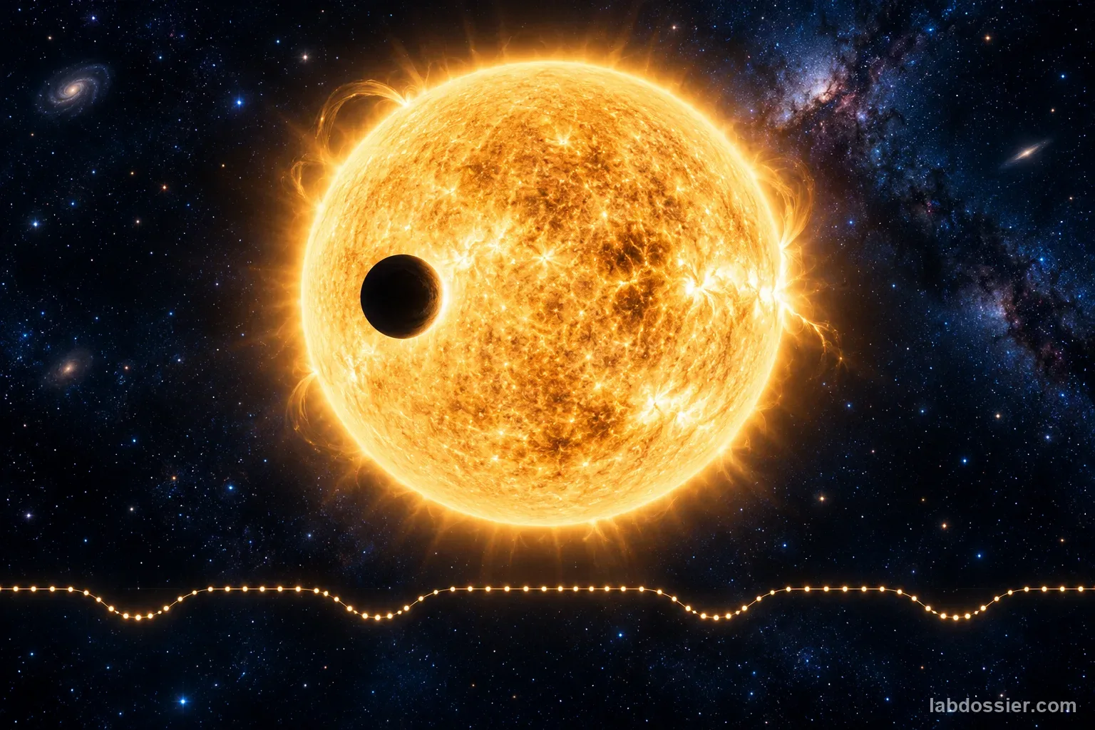
When a planet passes between its star and a telescope, it blocks a small fraction of the star's light. A time series of measured brightness is called a light curve. If similar dips repeat, their spacing can estimate an orbital period, while dip depth can constrain the planet-to-star size ratio under additional assumptions.
The signal can be tiny compared with measurement scatter. Real stars also vary, spacecraft can move, scattered light changes backgrounds, and data gaps can hide events. Detecting a pattern is a first inference step, not by itself proof of a planet.
10 // Plot time against normalized brightness
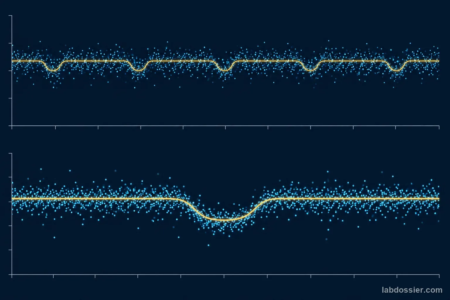
The table contains deliberately synthetic teaching values: three shallow dips were placed near an eight-hour rhythm, with small irregular changes added. Plot all 24 points in time order. The flux is normalized near 1.000, so 0.995 means about 0.5% below a unit baseline. Those values are fabricated to practice analysis and are not an observation from a named star.
A scatter plot leaves the individual measurements visible. It also makes missing samples and possible outliers easier to recognize. Avoid treating a line drawn between distant measurements as evidence that a telescope watched continuously during the gap.

11 // Fold the same curve at three trial periods
For a trial period P, phase = (t modulo P) / P. Measurements at the same phase from successive cycles can then be compared. At the injected eight-hour period, the synthetic dips align. At seven and nine hours they drift across phase because the trial clock runs faster or slower than the injected pattern.
Astronomers use methods such as Box Least Squares (BLS) to search a range of periods and transit durations for a repeating box-shaped decrease. A strong BLS peak proposes a period to investigate; it does not label the cause as a planet. The Lightkurve example walks through normalizing observations, finding a BLS peak, estimating period/epoch/duration and folding a known Kepler system.
12 // Estimate depth and compare scatter
Choose the phase interval that represents transit before comparing trial periods. Estimate the out-of-transit baseline from points outside the interval; estimate depth as (baseline − in-transit mean) / baseline. Report the number of measurements and their spread as well as the average. A dip supported by one point, or by only one cycle, is especially vulnerable to noise and chance alignment.
In real analysis, uncertainty depends on per-point precision, correlated noise, cadence, transit duration and the number of observed events. A simple classroom average is a comparison tool, not a formal detection significance or false-alarm probability.
13 // Test how noise removal can change the signal
NASA's TESS support tutorial explains that scattered light and instrumental systematics can remain in target-pixel or full-frame data, and compares cotrending, regression and pixel-level decorrelation methods. The correction must match the data product and timescale. A very short smoothing window may flatten a long transit; a long window may leave background drift or stellar variability.
Keep raw and processed versions and state the correction used. Compare whether the dip depth, timing and shape change. If the correction alters the candidate materially, treat that as uncertainty to investigate rather than choosing whichever plot looks most planet-like.
14 // Call it a candidate and list the next checks
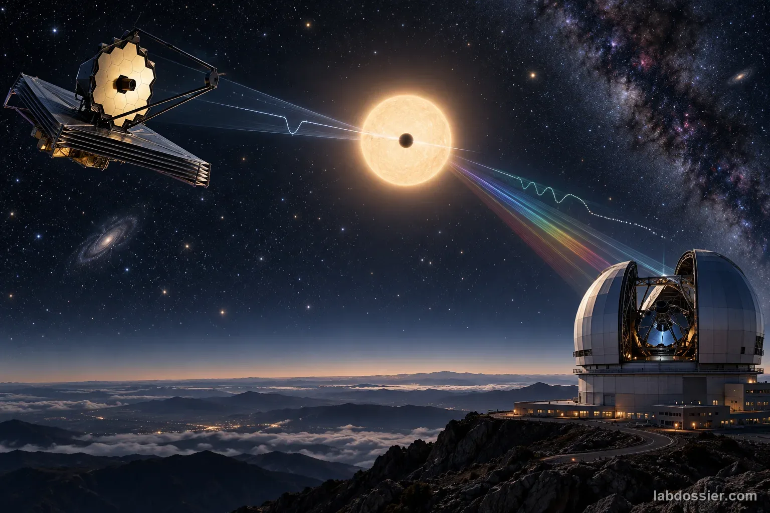
The NASA Exoplanet Archive separates transit-search events from planet candidates and supplies validation and vetting products. Its Kepler pipeline checks transit-like threshold events and promotes only some after further review. Data-validation tests examine whether an apparent signal is astrophysical or an instrumental or stellar false positive.
Common checks include odd-versus-even transit depths, secondary eclipses, pixel-level motion and centroid shifts, data-quality flags, stellar properties and independent observations. An eclipsing binary or blended background star can mimic a planet. Report a transit-like candidate and the evidence still needed; do not claim confirmation from this small synthetic set.
15 // Questions people ask
What does phase-folding do?
It wraps observations from different cycles onto one shared phase axis using a trial period. If the period is close to the repeat time of a transit, its dips can align and become easier to compare; the operation can also reveal when a trial period does not align them.
Why use a synthetic dataset?
It provides a known injected pattern for learning a method without implying that classroom analysis has discovered a planet. Real mission data have additional calibration, quality flags, gaps, stellar variability and instrumental systematics.
Does detrending always improve transit detection?
No. It may suppress slow instrumental variation, but an overly aggressive or poorly chosen correction can flatten a long or shallow transit. Compare raw and corrected series and explain the chosen timescale.
Can an eclipsing binary mimic a planet transit?
Yes. Stellar eclipses and blended sources can produce periodic brightness dips. Kepler's data-validation process uses diagnostic tests and follow-up metrics because transit-like behavior alone is not enough.
What is needed to confirm a planet?
Confirmation or validation uses evidence beyond a repeating dip, which may include pixel and centroid checks, odd/even comparison, secondary-event searches, statistical false-positive analysis, stellar characterization and independent follow-up observations.
16 // Keep going
Can you explain the investigation?
How can a repeating exoplanet transit be detected in a noisy light-curve dataset without mistaking it for proof of a planet? · Student Data Sheet
Question: Which trial period best aligns repeated shallow dips in a noisy synthetic light curve, and what evidence would still be needed before calling the signal a planet?
Hypothesis: If the same noisy measurements are folded at the period used to create their repeated synthetic dips, then the dips will line up at one phase and form a clearer average decrease than when folded at nearby incorrect periods, because phase folding places observations from repeated cycles at the same relative orbital phase, allowing a recurring pattern to reinforce while uncorrelated noise is less aligned.
Materials
- the 24-row synthetic flux table from this article
- spreadsheet or graph paper
- calculator
- phase-folding worksheet with candidate periods 7, 8 and 9 hours
Safety before starting
- The article's 24 values are synthetic. Keep that label with plots and exported files; do not post or present them as NASA or telescope measurements. When switching to real mission data, record the archive, target, data product and processing version.
- Use a trusted spreadsheet or astronomy package and avoid opening unknown scripts or data downloads. Do not remove points or modify the series only to create a stronger-looking transit; retain raw values and document every correction.
Lab notes
- All 24 table values are synthetic teaching data with an injected approximately 8-hour pattern. They are not measured values from Kepler, TESS, NASA, or any known star.
- Do not equate one dip or a strong periodogram peak with planet confirmation. Kepler validation products evaluate transit-like events with multiple diagnostic tests and false-positive checks.
- Detrending is a scientific choice: corrections can remove instrumental patterns but can also attenuate a real transit if the correction timescale overlaps the signal.
Variables
Independent: Trial period used to group the same time-ordered observations by phase · Dependent: How well a repeated shallow dip aligns in phase relative to the out-of-transit baseline
Keep constant: Use the same 24 time stamps and flux values, normalization, phase-bin width, transit window and candidate scoring rule; change only the trial period
Procedure
- Start with an explicitly synthetic dataset: Use the 24 time-and-flux values in the data table as if they were one short telescope sequence. The values are synthetic: a shallow dip was inserted near the same phase about every eight hours, then small scatter was added. Do not describe this table as a NASA observation or a real planet. Keep the raw values visible throughout the analysis.
- Plot time against normalized brightness: Make a scatter plot with time in hours on the horizontal axis and normalized flux on the vertical axis. Transit-like events appear as small decreases, not brightening. Mark uncertainty or outlying points; do not connect large gaps with a line that implies continuous observation. Note that the small visual changes are deliberately hard to see at first.
- Fold the same curve at three trial periods: For each trial period, calculate phase = (time modulo period) ÷ period. Use the same phase bins for all three tests and calculate the mean flux in each bin. Compare whether the lowest points cluster at one phase across multiple cycles. An eight-hour period is the injected pattern, but students should justify it by alignment, not by being told the answer before plotting.
- Estimate depth and compare scatter: Choose the in-transit phase window before scoring periods. Estimate transit depth as the out-of-transit baseline mean minus the mean inside that window, expressed as a fraction of baseline. Also report the number of points and their spread; a deeper apparent dip based on one point or one cycle is weaker evidence than a repeated, aligned pattern. Do not silently remove data to improve the score.
- Test how noise removal can change the signal: For a real Kepler or TESS light curve, slow instrumental trends, scattered light, stellar rotation, flares and gaps may require correction. Compare the raw and corrected series and preserve a copy of each. A detrending window that is too short can flatten or erase a long or shallow transit; a window that is too long can leave background trends. NASA's TESS tutorial compares correction methods because no one correction is right for every star and timescale.
- Call it a candidate and list the next checks: A repeating dip is a transit-like candidate, not proof of a planet. Eclipsing binary stars, blended background sources, stellar variability, instrumental events and data-processing artifacts can mimic or distort a signal. Professional vetting examines the pixel data, odd/even events, secondary eclipses, centroid shifts, statistical significance and follow-up observations. Report the method, assumptions and uncertainty before making a claim.
Record your observations
| Time (h) | Synthetic normalized flux | Time (h) | Synthetic normalized flux |
|---|---|---|---|
Compare candidate periods using the same scoring rules
| Trial period | Expected phase result | What to report | Caution |
|---|---|---|---|
A transit-like dip has several possible causes
| Possible cause | Why it can look transit-like | Useful follow-up |
|---|---|---|
Answer key and expected pattern
The 8-hour folding best aligns the synthetic dips near the same phase; the 7- and 9-hour trials spread them more broadly.
The estimated depth is small compared with baseline flux, so plotting, repeated events, noise and selected phase windows matter to interpretation.
The data demonstrate recovery of a deliberately inserted signal only. A real transit-like signal needs pipeline vetting and follow-up before it can be described as a confirmed planet.
Remember: A repeating dip can reveal a candidate transit, but other stars and instruments can imitate the same pattern. Show the raw light curve, state how you normalize and fold it, compare nearby trial periods, preserve possible transit signal during detrending, and separate candidate detection from confirmation.